Code a program to solve a partial differential equation using finite differences with an explicit method

The goal of this post is to create a program to solve a differential equation in 2D. I will present the programming in C++ but the concepts here are easily translated to other languages. I myself have used Julia a couple times. The equation that we are going to solve is the Poisson equation with Dirichlet boundary conditions in a $1\times 1$ square. The equation and the conditions are given by

\begin{aligned} \nabla f(x, y) & = u(x, y), \\ f(0, y) & = g(0, y), \\ f(1, y) & = g(1, y), \\ f(x, 0) & = g(x, 0), \\ f(x, 1) & = g(x, 1). \end{aligned}

Internal points

Before coding anything, we need to expand the $\nabla f(x,y)$ term using finite differences on it. To expand the term is quite easy and results in \begin{aligned} \nabla f(x, y) &= \frac{\partial^2 f}{\partial x^2} + \frac{\partial^2 f}{\partial y^2}. \end{aligned}

Finite differences is a method that allows us to remove the continuous $x$ and $y$ variables to introduce discrete variables $i$ and $j$ which will be used to iterate in a loop. This is an approximation and the accuracy increases with the number of discrete points one wants to use, but makes the implementation more complicated as well as costs more computing power. To discretize a second order partial differential term with second order accuracy, we have the relation

\begin{align} \frac{\partial^2 f}{\partial x^2}(x, y) &\approx \frac{f(x_{i-1},y_i)-2f(x_{i}, y_i)+f(x_{i+1},y)}{\Delta x^2}, \end{align}

where $\Delta x = \mathrm{span}(x)/N$ and $N$ is the number of points that a given dimension has. Remember that the continuous variable $x$ has infinite points, but when we use $x_i$ we use only a finite set of points of size $N$. The number of points $N$ will be same for both dimensions, so we have $\Delta y = \Delta x$.

Regarding $u(x,y)$ we just evaluate it at $(i\Delta x, j\Delta x)$. This way, we have our discrete equation

\begin{align} c_{ij} = \sum_{m=-1,1}f(x_{i-m}, y_i) + \sum_{n=-1,1}f(x_i, y_{j-n}), \\ \frac{1}{\Delta x^2}\left(c_{ij} - 4f(x_i, y_i)\right) = u(i\Delta x, j\Delta x).\label{eq:discretizedPoisson} \end{align}

Notice that Equation \eqref{eq:discretizedPoisson} is our discretized Poisson equation. As the focus of this post is to present code using an explicit method, we isolate the term $f_{ij}$ like in

\begin{align} f_{ij} &= \frac{c_{ij}}{4} -\frac{u_{ij}\Delta x^2}{4}. \label{eq:internalPoints} \end{align}

We can use Equation \eqref{eq:internalPoints} for any point internal to our $1\times 1$ square. Nevertheless, for the boundary points, i.e where $x\in {0,1}$ or $y\in{0,1}$, we can not use it as we will not be able to compute $i-1$, $i+1$, $j-1$ or $j+1$. I mean, these points would be outside our mesh.

Boundary points

Regarding the boundary points, it is super easy with Dirichlet conditions. We will just do

\begin{align}f_{ij} = u_{ij}. \label{eq:boundaryPoints}\end{align}

Code

With Equations \eqref{eq:internalPoints} and \eqref{eq:boundaryPoints}, we can finally code a simple solution to solve our Poisson equation. Notice that I am testing this code with g++ 6.2.0. I will present the main functions as well as some of the utility functions I did.

Regarding utilities, I used a timer class, so that we can compute how long this method takes, an abs function, so that I know the absolute differences between iterations, and a getMesh function to allocate memory and give me a pointer. These three functions are presented in

class Timer
{
public:
    Timer() : beg_(clock_::now()) {}
    void reset() { beg_ = clock_::now(); }
    double elapsed() const {
        return std::chrono::duration_cast<second_>
            (clock_::now() - beg_).count(); }

private:
    typedef std::chrono::high_resolution_clock clock_;
    typedef std::chrono::duration<double, std::ratio<1> > second_;
    std::chrono::time_point<clock_> beg_;
};


double abs(double x) {
  if(x < 0) return -x;
  return x;
}

// Remember we are considering number of points in x == y
double ** getMesh(int n) {
  // we use calloc to initialize everything with zeros
  double ** mesh = (double**) calloc (n, sizeof(double*));
  for (int i = 0; i < n; i++) {
    mesh[i] = (double*) calloc (n, sizeof(double));
  }

  return mesh;
}

The boundary conditions need to be computed only once and it depends on the function $g(x,y)$ that we pass as an argument to another function:

/**
  g is a function of (x,y) that is applied on the boundaries
*/
void computeBoundaries(double ** mesh, int n, function<double(double, double)> g) {
  int i, j;
  double dx = 1 / (n - 1);
  i = 0;
  for (j = 0; j < n; j++) mesh[i][j] = g(i * dx, j * dx);
  i = n - 1;
  for (j = 0; j < n; j++) mesh[i][j] = g(i * dx, j * dx);
  j = 0;
  for (i = 0; i < n; i++) mesh[i][j] = g(i * dx, j * dx);
  j = n - 1;
  for (i = 0; i < n; i++) mesh[i][j] = g(i * dx, j * dx);

  return;
}

For the internal points, we do something similar by accepting a function as argument

/**
 f is a function that expects mesh and i, j and computes the value of
 that point. It also takes the absolute change reference and adds to it.
 The return of this function is the absolute change
*/
double computeInternalPoints(double ** mesh, int n, function<double(double**, int, int, double*)> f) {
  double absoluteChange = 0.0;
  // only internal points, that's why there is the loop goes from 0 to n - 2
  for (int i = 1; i < n - 1; i++) {
    for (int j = 1; j < n - 1; j++) {
      mesh[i][j] = f(mesh, i, j, &absoluteChange);
    }
  }

  return absoluteChange;
}

Now, having these functions, the main idea is simple: run computeInternalFunctions as long as absoluteChange is smaller than a threshold. In math representation, this can be

\begin{align} \sum_{i}\sum_{j} |\mathrm{mesh}{ij} - \mathrm{mesh}^*{ij}| < \epsilon, \end{align}

where $\epsilon$ can be pretty small but increases the computation time for the function to converge, i.e. the time for the program to get a solution. The variable $\mathrm{mesh}^*$ is the variable $\mathrm{mesh}$ after all its internal points were computed again by the function passed to computeInternalPoints.

The final code in C++ as well as code to plot it (in python) is available here. If you look at the code, I hardcoded the Dirichlet conditions there, but you can change it to your liking. To compile and plot it, I do the following:

$ g++ -std=c++14 poissonDirichlet.cpp -o solver_dirichlet
# run with a mesh of size 100 and output file is at out.bin
$ ./solver_dirichlet 100 out.bin
Finished computing! Latest absolute change was: 9.99971e-05
Total number of iterations on mesh: 9497
Total time spent: 4.71717 seconds
Total time per iteration: 0.000496701 seconds
File size: 80004 bytes
File successfully saved at: out.bin
# use python to plot the result on the screen
$ python plot.py --filename out.bin

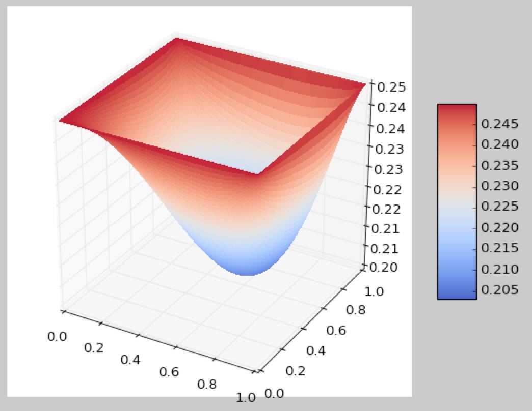
The final result is

Notes

This is not the most efficient implementation to solve but it is a good starting point for whoever is starting. If you were curious about how time goes on as we increase $N$, you can just check at this table:

Thanks for reading! If you have any questions or suggestions, let me know! You can comment, send me an e-mail, whatever suits you!